
We use auto filters to filter subsets of data in Excel, but this filtering is limited to actual data. We can use Advanced Filter feature to filter multiple columns with different criteria.
Understanding with an example will be easy.
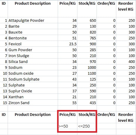
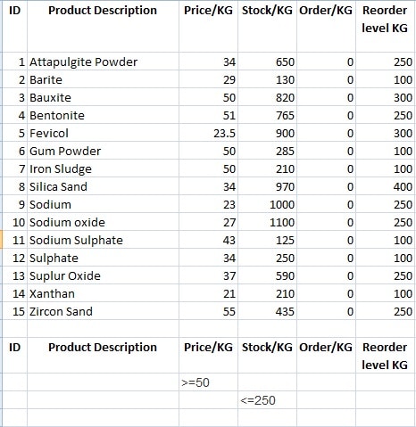
Open a workbook in Excel and copy below data into the sheet.
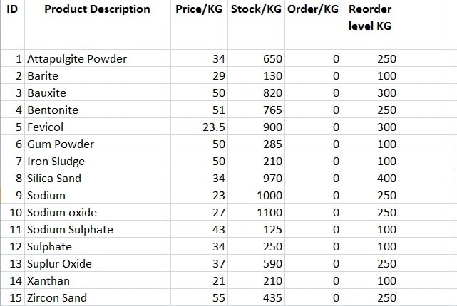
You can also use your own dataset instead of this data.
Click here to download the workbook sample data.
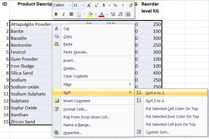
I have used the simple sorting feature of Excel to sort the data alphabetically.
To sort your data alphabetically, select the data and right click the mouse. From the menu select “Sort” option and select “Sort A to Z”. It will sort your data alphabetically.
Shortcut Key for sorting data alphabetically: Function key + O + S
See below image for reference:
Simple Filter
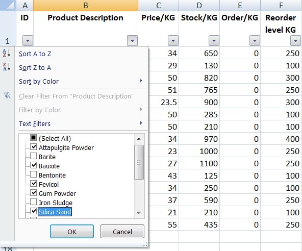
To filter the data on an actual basis, select the headings of your data. Go to Data Tab > Sort & Filter> Select Filter.
Each column will have a drop down list. Select your relevant options to filter multiple columns according to your need as shown in below image.
Simple filtering has its limitations and thus to filter multiple columns with multiple criteria you need to use the Advanced Filter feature.
You can use Advanced Filter feature with AND and OR operators to create complex filtering combos.
Let us apply AND and OR operators on this example one by one.
Filter Multiple Columns With Multiple Criteria
For using the Advanced Filter feature we need 2 things:
- List Range
- Criteria Range
1. Advanced Filter with AND operator
Copy the headings of the data either to another area on the same sheet or onto a different sheet.
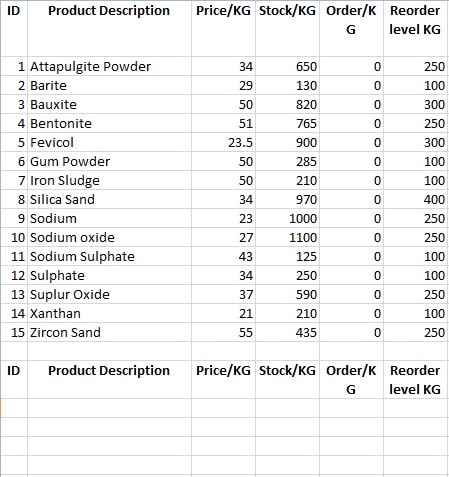
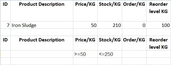
Suppose we want to know the products that have a price range of Rs. 50 or more and have 250 or more kilograms in stock. Filtering the data here requires satisfying both the criteria.
Enter >=50 in Price column and <=250 in Stock column as criteria.
Note: While using AND criteria should be mentioned in the same row.
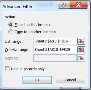
Click on Data Tab> Sort & Filter > Advanced.Below dailog box will appear.
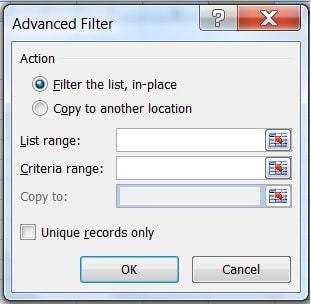
Retain the default setting, Filter the List In-Place.
Enter List Range. List range is the data range. In our example, it is Sheet1!$A$1:$F$16.
Enter Criteria Range. Criteria Range will be Sheet1!$A$18:$F$19.
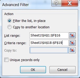
Click “OK”. You will get the result of filtering as shown below.
1. Advanced Filter with OR operator
Filtering data with OR operator we need to fulfill either of the criteria.
Note: Insert the in a different row to use OR operator.
Enter List Range. List range is the data range. In our example, it is Sheet1!$A$1:$F$16.
Enter Criteria Range. Criteria Range will be Sheet1!$A$18:$F$20.
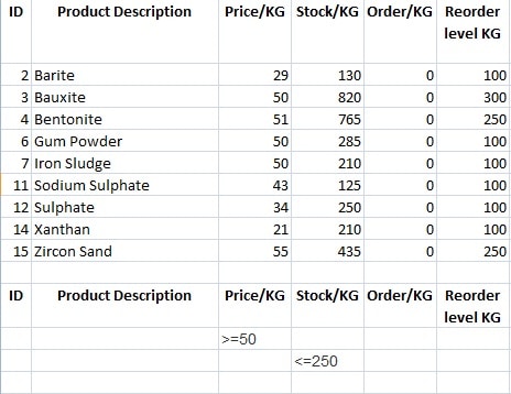
Click “OK”. You will get the result of filtering as shown below.
To learn more about Advanced Filtering click on the link below:
Additionally, you can download other accounting templates like Petty Cash Book, Simple Cash Book, and Accounts Payable Excel Templates from here.
We thank our readers for liking, sharing and following us on different social media platforms.
If you have any queries please share in the comment section below. I will be more than happy to assist you.