There is a myth related to creating a drop-down list in excel. It is often considered something hard and only for professionals. I myself had such silly conception when I started learning excel about a decade ago. No, it is not at all correct.
You can create a Drop-down list in just 3 easy steps which might take about 30-40 seconds of your time. It might seem weird but it’s really that easy.
Steps to Create a Drop-down List
Open your workbook in which you want to enter the drop-down list and follow the steps given below:
1. Press Alt + A + V + V which is the keyboard shortcut for Data Validation. The Data Validation window appears.
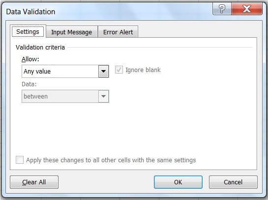
You can do the same by a long process also. In the Ribbon go to Data Tab, in the Data tools select Data Validation.
I personally prefer to use the keyboard shortcuts. These shortcuts help you save time and projects you like a professional in front of your colleagues.
2. On the Settings tab, in the Allow box, click List.
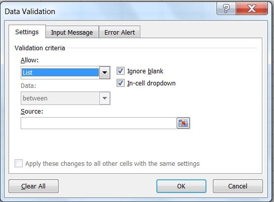
3. In the Source Box either select the data from your desired sheet. You can directly type into the source box if the list you want to create is just yes/no, a/b/c/d.
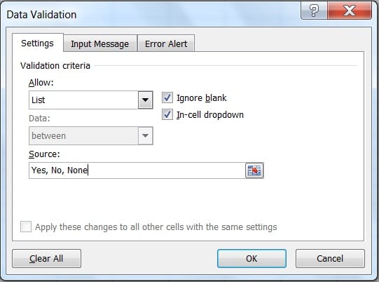
In other words, you need not have to create a special table for data to insert in the drop-down list.
Your dropdown list is ready. Isn’t it simple?
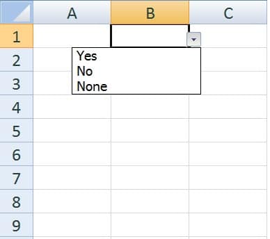
Above, we discussed how to create a simple dropdown list. You can also make a drop-down list with advanced data validations such as it accepts only a numbers or text, to display a warning message when data doesn’t match etc.
Let us create a drop-down list with advanced data validations.
Before we proceed to start the process of creating a dropdown list we need some data of which we will create the list from. We will try to create a drop-down list of employees of a company.
First and foremost, write the names of the employees in column A of your sheet. Sort the data according to the type of data, either alphabetically or numerically.
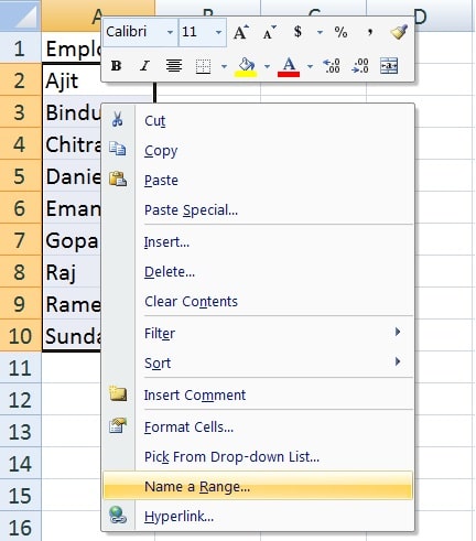
Secondly, select the data, right-click, and then click on “Name a range”.
In the Name box, give a name according to your data. Here we will give the name to the range as Employees.
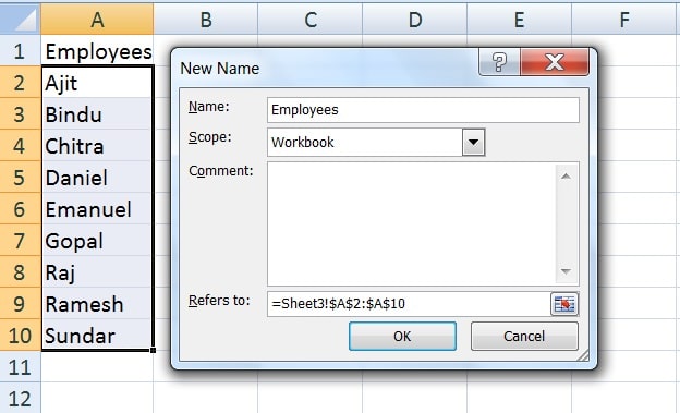
Make sure that name of the range should not contain any spaces. If there are two words write them without space. You will not be able to link this range if the name of the range contains a space.
Drop-down List with Input message and Error Alert
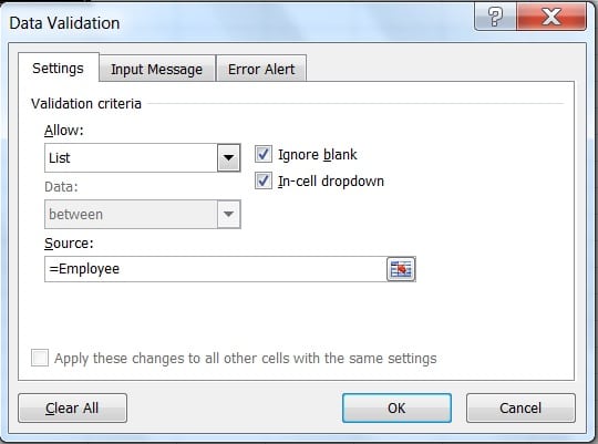
Press Alt + A + V + V which is the keyboard shortcut for Data Validation. The Data Validation window appears.

On the Settings tab, in the Allow box, click List.

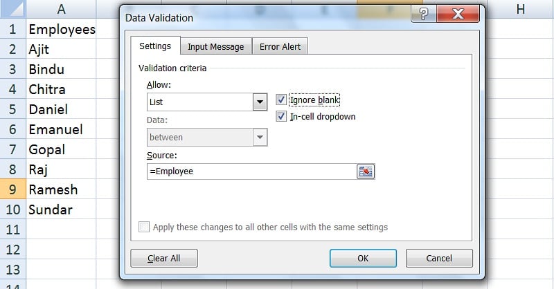
Check both the boxes beside the Allow box, Ignore blank and In-cell dropdown.
In Source box, type equal sign (=) followed by the name of the range that we have given to it earlier. Our range name is “=Employee”.
Go to Input tab if you want to enter a popup message when the cell is clicked. Check the “Show input message when cell is selected.”
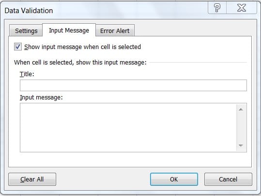
Type the input message you want to display.
You can uncheck the box if you don’t want any message to be shown when cell is clicked.
Users can also put an Error Alert if the data entered is invalid. To do this Go to Error Alert tab.
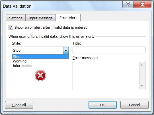
Check the box beside “Show error alert after invalid data is entered”. Choose an option from the Style box which you find appropriate for you. Type a title and message you want to display.
You can uncheck the box if you don’t want any message to be shown when there is an error.
Your employee list is ready.
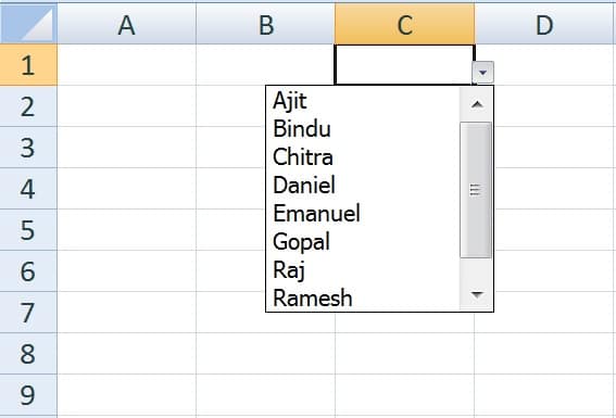
Hope I was able to clear the myth and ease te work excel users.
We have created infographics for Excel Functions. You can learn step by step how to use different functions of Microsoft Excel.
Additionally, you can download other accounting templates like Break Even Analysis Template, Salary Sheet Template and Invoice with GST Template from here.
Visit our Templates page for a wide range of Excel Templates for Accounting and Analysis purposes. These templates are free, customizable and easy to use.
We thank our readers for liking, sharing and following us on different social media platforms.
If you have any queries please share in the comment section below. I will be more than happy to assist you.