RANK function is used to compare numbers to other numbers in the same list. RANK function will tell you the rank of a given number from a range of number in ascending or descending order.
Syntax
=RANK(number or cell address, ref, (order))
This function is used at various places like schools for Grading, Salesman Performance reports, Product Reports etc.
Let’s understand it better with the help of an example.
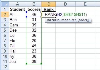
We have a list of 10 students and their test scores from cell B2 to B11 as shown below:

To find the rank of the first student’s score in cell B2, enter this formula in cell C2:
=RANK(B2,$B$2:$B$11)
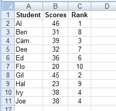
Just double click the fill handle and it will copy the formula from cell C2 down to cell C11. The scores will be ranked in descending order as shown below:

Arguments of RANK Function
There are 3 arguments for the RANK function:
- Number or cell address: In our example above the number to be ranked is in cell B2.
- Ref (range): We want to compare the number to the list of numbers in cells from B2 to B11.An absolute reference will be used ($B$2:$B11) instead of a relative reference (B2:B11), so that the referenced range doesn’t change when we copy the formula to the cells below.
- Order: This argument is optional. This argument will tell Excel to rank the list in ascending or descending order as required.
Ranking in ascending or descending order
Using 0 (zero) or leaving this argument empty will give the ranks in descending order.
In our example, we left the order argument blank in order to find the rank in descending order.
The formula used is =RANK(B2,$B$2:$B$11)
For ranking them in ascending order, we need to type 1, or any other number except zero.
For comparing golf scores, we could type 1, to rank in ascending order.
=RANK(B2,$B$2:$B$11,1)
A question might arise here that what will happen to the ranking if some of the scores are similar in other words scores tie with other scores?
Microsoft Excel will automatically skip subsequent numbers to show the correct rank.
As we can see in our example, the last two scores in the list are the same. Both the students Ivy and Joe are ranked as 4th.
The score for Ed is 36. Excel has ranked it 6th instead of 5th because there are 5 students ahead of Ed, two of them having 4th rank.
If you have any queries please post them in comments. I will be more than happy to help.
i used the same rank command to rank the students passed in exam but the final rank is increased by one number(i.e, it should be 8 instead it shows 9). i dont know why can you clarify me.
It seems that there might be an issue in the formula. Either copy and paste the formulas here so that I can see or send me file on my email.
Dear sir thanks for your reply. i cant see your mail id to send the file.
This is the formula i used to calculate the rank
=IF(AND(D2>34,E2>34,F2>34,G2>34,H2>34,I2>34),RANK(J2,$J$2:$J$37,0),”–“)
it checks six subject marks >34 then it ranks according to the total
info@exceldatapro.com
i am waiting for your reply sir