Today I will show you how to round up values using ROUND, ROUNDDOWN, and ROUNDUP functions.
Using the above functions for rounding will change the value of the number and the display of the number in the worksheet as per the given argument.
Let’s understand each in detail with relevant examples.
ROUND Function
ROUND function rounds a given number to a specific number of decimal places as per our requirement. It contains two arguments, the cell reference or a number and the number of decimal places required.
Syntax: =ROUND(number, num_digits)
The number argument can be a number, a cell reference that holds a number, or a formula which results in a number format.
The num_digits argument can either be a negative or a positive integer. If we use a negative number it rounds that number of places to the left of the decimal point. If we use 0 (zero), it rounds to the nearest whole number.
The number less than 5 in the decimals get rounded down and the numbers that are 5 or more than 5 in the decimals get rounded up according to the basic mathematic principle.
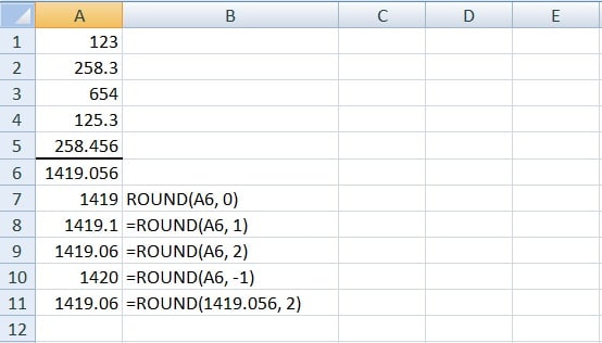
In the image below we have some numbers with decimal values in cell A1 to A5. As we sum the total of all it gives the result as 1419.056.

The formulas applied to each cell in column A are mentioned in column B, so it becomes easy to understand and apply the formulas as per our requirement.
We can also use a number as the Number argument as shown in the last formula in the figure.
ROUND DOWN
ROUNDDOWN function is same as ROUND but this function rounds the number down.
Syntax:=ROUNDDOWN(number,num_digits)
As shown below make slight changes in numbers and apply the ROUNDDOWN function we get the results as shown in the screenshot:
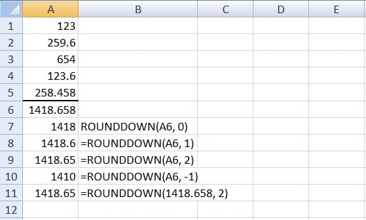
The formulas applied to each cell in column A are mentioned in column B for you to understand it better.
Just as ROUND function, we can also use a number as the Number argument as shown in the last formula in the above figure.
ROUNDUP Function
ROUNDUP results are just the opposite of ROUNDDOWN. It rounds the number upward.
Syntax for ROUNDUP
=ROUNDUP(number,num_digits)
Taking the first example and applying the ROUNDUP function, give you the results as shown below:
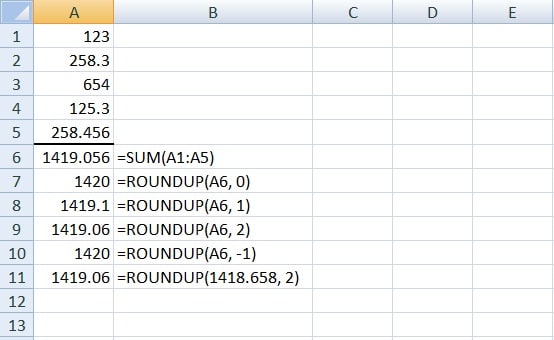
We can even apply the syntax for ROUNDUP with the number rather than using cell address like ROUND and ROUNDDOWN functions.
We can use all the above rounding functions with other functions. For example, we need to use it with SUM function. The only change make is in the syntax.
Instead of cell reference or number we need to put the formula in the syntax. I have applied the ROUND function along with SUM formula in the image below:
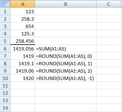
Similarly, we can use it with ROUNDDOWN and ROUNDUP functions also.
Share your comments and queries and I will be happy to assist you.