
List of Functions
- SUM Function
- Count Function
- CountA Function
- LEN Function
- TRIM Function
- RIGHT, LEFT and MID Function
- VLOOKUP
- IF Statements
- SUMIF, COUNTIF, AND AVERAGEIF
- CONCATENATE Function
1. SUM Function
The SUM function allows you to add 2 or more numbers together. Sum function can be directly applied to sets of numbers separated by a comma, two or more cells separated by comma or selecting a range of cells. Let us discuss it in more detail.
1. Adding 2 or more values/cells separated by a comma:
First, let us understand adding 2 or more numeric values separated by a comma. For example, let us add 25+35+24.
In the Excel sheet put the equal sign and then write SUM and open a bracket and put above three values separated by a comma and then close the bracket and press enter. Excel will calculate and give us the total.
Formula: =SUM(25,35,24) Answer: 84
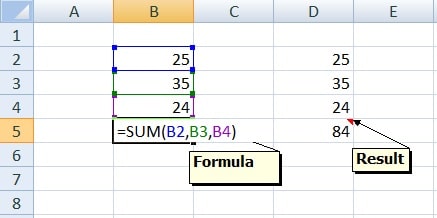
For using SUM formula for two or more cells separated by a comma instead of putting numeric value us need to put cell. =SUM(B2,B3,B4).
For reference see the screenshot below:
2. Adding a range of cells :
As I explained above how to use SUM function for two or more numeric values and cells separated by a comma and now let us discuss to use SUM function for a range of cells.
The keyboard shortcut for using SUM function for a range of cells is Alter + Equal (ALT + =). Press both together and it will automatically add the whole range of cells above the formula. We can also select range as required.
See figure below to understand it:
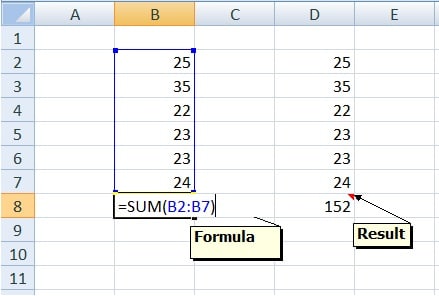
Formula: =SUM(B2:B7) Answer: 152
The range of cells here is B2 to B7. It is separated by the “: ” sign.
2. COUNT Function
The count function counts the number of cells containing numbers for a selected range. This formula only works with numbers. It counts the cells where there are numbers. The formula for the count is =COUNT(Cell Start: Cell End).
We can see the difference in the below image. On the left side, the result of the formula is 10 and on the right side, the same formula shows the result as 9 because on the right side one cell contains the text.

3. COUNTA Function
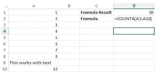
This function counts the number of non-empty cells in a selected range. It will count cells that have numbers and/or any other characters in them.
Formula: =COUNTA(A1: A1O)
It counts the number of non-empty cells no matter whatever the data type maybe.

4.LEN Function
The LEN formula counts the number of characters in a cell including spaces.
Formula: =LEN(B3)
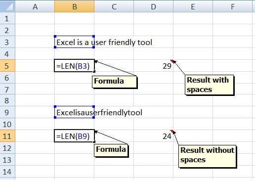
Notice the difference in the formula results. 24 characters without spaces in between the words, 29 with spaces between the words.
5. TRIM Function
This TRIM function is useful for removing extra spaces in a cell whether at the beginning, trailing or anywhere between the words.
Often when you pull data from a database you may find some extra spaces are put in behind or in front of legitimate data.
This can create huge discrepancies if you are trying to compare using IF statements or VLOOKUP’s.
Formula: =TRIM(A1)

I added an extra space behind “I Love Excel”. The TRIM formula removes that extra space. Check out the character count difference with and without the TRIM formula.
6. RIGHT, LEFT and MID function
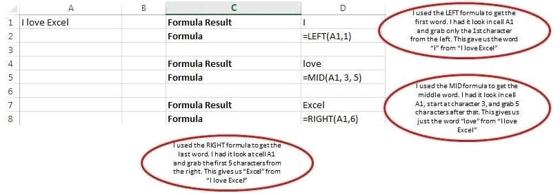
These RIGHT, LEFT and MID functions return the specified number of characters from a text string.
RIGHT gives you the number of specified characters from the right of a text string. LEFT gives you the number of specified characters from the left of a text string. MID gives you the number of specified characters from the middle of a text string.
- =RIGHT(Text or Cell reference, number of characters you want to look for)
- =LEFT(Text or Cell reference, number of characters you want to look for) and
- =MID(Text or Cell reference, Start Number, number of characters you want to look for)
7. VLOOKUP Function
VLOOKUP Function is the most used function in day to day operations of many businesses.
It looks for a particular value in another table or array and returns the value in the same row from a specified column.
In simple terms, it does a find action of a value from one sheet or table or file in another sheet or table or file and copies the value corresponding to that value from the column specified in the formula
Formula: =Vlookup(lookup_value, table_array, col_index_num, range_lookup)
The above formula has 4 parts as described in the formula:
Lookup_Value: This is the field that has common references or values to another file which has more details
Table_Array: This is the range that we select from another file or sheet or table starting from the column which has common references/values to the lookup_value as defined above.
Col_index_num: This is the column reference number from which you wish to pick values against the lookup value as defined above.
Range_lookup: This is used to derive an approximate or exact match. “0” or “False” value will provide an exact match whereas “1” or “True” value will provide an approximate match.
We can understand it with an example. See image below
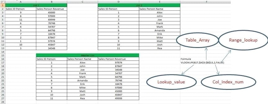
We are attempting to create a Master List from List 1 and List 2 using Sales ID Person as our “Lookup _value”.
Some important points to remember while using the VLOOKUP function.
- For a VLOOKUP function, there always needs to be a common field with common values which is referred to as “lookup value”.
- To understand VLOOKUP better we should keep this in mind that we give the command to excel to lookup “x” in this range i.e. “x:y” and pick up “y” and do an exact match by “False” or “0”.
8. IF Statements
IF Statement is also among the most used formula for analytical scenarios, where a data has to react differently based on different situations
Formula: =IF(logical_test, value_if_true, value_if_false)
Logical Statements may include a comparison of one value to another using “>‘ “<‘ “=‘ “OR’ “AND”, etc.
IF Statement formula is divided 3 parts:
Logical Statement: It is usually a comparison statement using Logical Operators.
True value: If the answer to the logical statement is true, the value specified for true value will be returned
False Value – If the answer to the logical statement is false, the value specified for false value will be returned
For Example:

“IF Statement” is a very powerful formula that is used to derive results of complex problems. It avoids using multiple steps while working on a worksheet and gives results in one shot. This can be done using Nested IF Statements.
Example of a Nested IF Statement
Formula: =IF(logical_test, value_if_true, if(logical_test, value_if_true, if(Iogical_test, so on and so forth)
Nested IF always has a new IF Statement for each False value. This formulation can be continued until all the situations are covered. This statement is very useful for teachers, academic heads, and also defining Age Buckets.
For example, IF we want to define an age group, below apply the below given IF Formula
=if(age<7, “0-7”,if(7<age<15, “8-15”, if(15<age<30, “16-30”, if(30<age<60, “31-60”, “60 and above”))))
There is one IF Statements named as IFERROR
This formula will be triggered if the other formulas end up giving an error. It can look something like #N/A and that’s pretty ugly. This can happen for many legitimate reasons, but if we don’t want to hand a sheet full of #N/A symbols to our department heads then this function is useful.
In the above example to avoid #N/A values we can put formula as below:
=IFERROR(if(age<7, “0-7”,if(7<age<15, “8-15”, if(15<age<30, “16-30”, if(30<age<60, “31-60”, “60 and above”)))),”“)
9. SUMIF, COUNTIF, AND AVERAGEIF
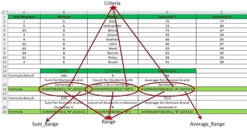
SUMIF, COUNTIF, and AVERAGEIF are used when more than one condition is fulfilled for a particular result. For example a Grade Sheet, Report Cards of Schools, Sales Performance reports, Analytical surveys, etc. These Formulas do their respective functions i.e. if the criteria are met.
=SUMIF(Range, Criteria, Sum_Range) provides the sum of values within cells IF the defined criteria are fulfilled.
=COUNTIF(Range, Criteria) provides a count of cells within cells IF the defined criteria are fulfilled.
To understand in detail how COUNTIF can be used to compare two data sets click the link below:
How To Use COUNTIF() To Compare Two Data Sets?
=AVERAGEIF(Range, Criteria, Average_Range) provides an average of the values within cells IF the defined criteria are fulfilled.
Please see the image below to understand the above statements.
10. CONCATENATE
CONCATENATE is a simple yet very effective and useful function for many day-to-day operations in an office. This Function is also denoted by Ampersand (&) Sign and it is used for joining the values in different cells.
Many times, we get a database where we feel the need to combine 2 columns or 2 fields; this formula helps to achieve that in no time.
For example, see the screenshot below which contains First name, Middle name and Last name of a group of people. To write all three together in one column CONCATENATE is very useful.

I have used CONCATENATE function in Column D to derive Full Names from the information given in Columns A, B and C
Formula: = Concatenate(A2,” ” ,B2,” ” , C2) OR =A2&” “&B2&” “&C2.
In the above formula, I have combined the First Name, Middle Name, and Surname with Spaces between each of them. SPACE or any Text which has to be put in between has to be denoted in “Quotation” Marks to be reflected in the result.
If you have any queries please write them in comments. I will be happy to reply.